| docs | ||
| include | ||
| lib/glfw | ||
| src | ||
| .gitignore | ||
| CMakeLists.txt | ||
| README.md | ||
Computer Graphics Lab4 - GPGPU in OpenCL
Deadline: Nov. 29 2024, 22:00
Instructions on how to build the project can be found here.
On Thursday November 22, during the lecture, a brief introduction of OpenCL will be given, and the slides (e.g. CG_Lab4_GPGPUinOpenCL.pdf) will be made available on Ufora. Definitely check those out once they are online.
Introduction to GPGPU programming
General-purpose computing on GPUs (GPGPU) means that the task at hand is typically performed on one or more CPUs, but is run on one or more GPUs. This allows programmers to take advantage of the massive number of parallel cores to significantly speedup calculations. An overview of important applications can be found here.
Several APIs exist, such as OpenCL, CUDA, DirectCompute and Halide. In this assignment, we will be using OpenCL, since many PC platforms offer implementations of the standard (AMD, ARM, Intel, NVidia, etc.).
Note: OpenCL is a native C library. Your implementation will use a C++ OpenCL wrapper, which means all required functions reside in the cl:: namespace.
In this lab, you will implement 2 applications:
-
A perlin noise texture generator.
-
A simplified fluid particle simulator.
This lab also uses OpenGL to visualize your OpenCL results. On Linux, install the following packages if this was not already the case:
sudo apt install libgl1-mesa-dev
sudo apt install freeglut3-dev
Assignment 1: Perlin Noise texture
Perlin noise is a type of procedural noise that is often used within computer graphics applications. In contrast to blue noise, perlin noise textures are smoother and the visual details are all the same size. This allows different layers of scaled (and rotated) perlin noise to be stacked to create interesting textures. For example, perlin noise is used for terrain height maps, or the transparency of clouds, or the curl direction of fur, or the organic blending of other textures.
1 Background
Perlin noise is a type of noise first published by Ken Perlin in a SIGGRAPH paper in 1985. At that time, he was working on the computer-generated effects for Disney’s Tron(1982). Perlin was dissatisfied with how “machine-like” the effects looked in that film, and started developing his idea of using textures, specifically natural looking ones.
Back then, the norm was traditional texture mapping, where an image is stored in RAM and sampled from using texture coordinates, which are associated with the three-dimensional (3D) vertices of a triangle mesh.
Perlin noise started the rise of procedural textures, which are created from noise and mathematical expressions. This has several benefits. Firstly, no image needs to be stored in memory, since the texture can be generated on the fly. This was great in the 1980s where computers only had a couple of KB of RAM. Secondly, there is no need for texture mapping if the expressions allow for 3D or even 4D inputs.
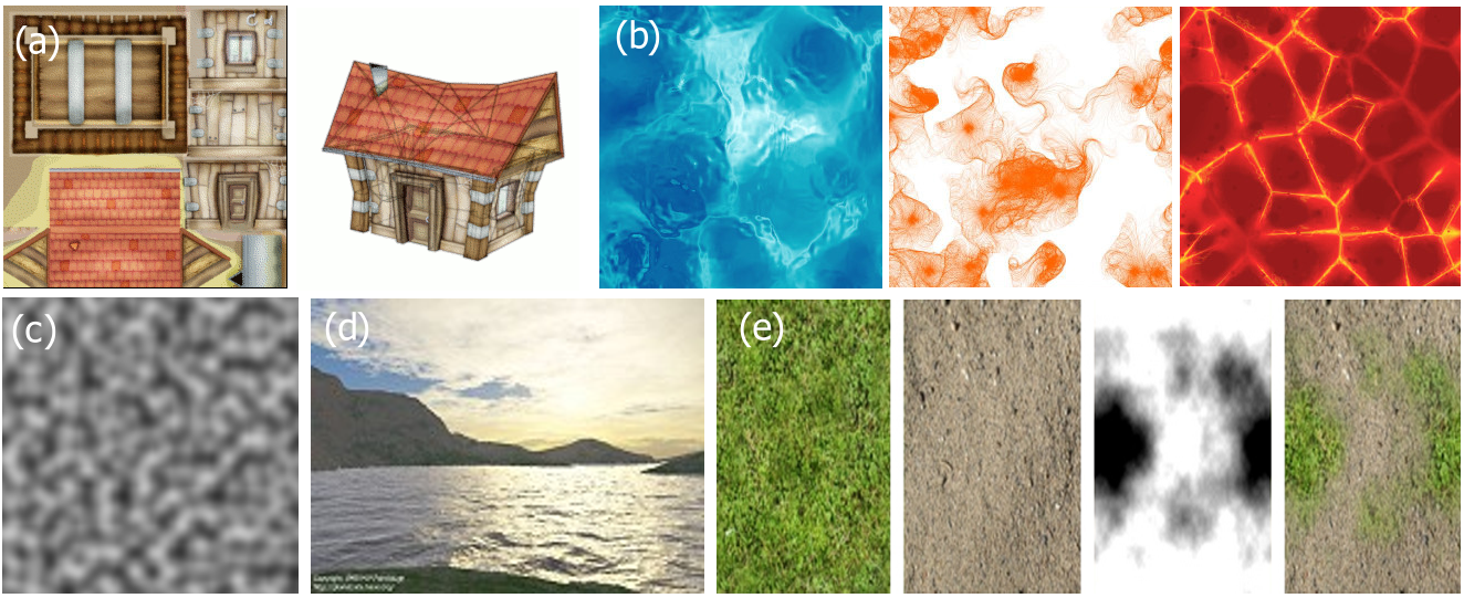
(a) Traditional texture mapping. (b) 2D slices of procedural textures. (c) 2D slice of 3D perlin noise. (d) Clouds, terrain and water ripples created using layers of perlin noise. (e) The blending of two image textures done by a (layered) perlin noise texture.
2 Basic idea
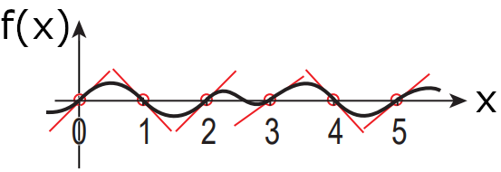
The graph below shows an example of 1D perlin noise f(x). An array of equidistant points is created from the whole integers along the X-axis (in 2D, this would be a grid). In these points, a pseudo-random gradient (slope) is chosen. f(x) results from a smooth interpolation between these gradients. This is the basic idea of perlin noise.
3 Original implementation
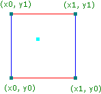
Perlin noise can be calculated in 1D up to 3D and even 4D, but in this assignment we will focus on 2D perlin noise to create an image texture. In other words, the input to the algorithm is a 2D point P = (x, y). In the figure below, P is a cyan dot. Notice how P lies between 4 corners of the 2D grid of integers x0, y0, x1 and y1.
Question: if for example
P = (x,y) = (2.3, 4.8), what are the values ofx0,x1,y0andy1?
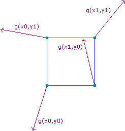
For each of the 4 corners, a pseudo-random gradient vector is calculated through function g, which is explained in Section 2.3.1. For example, the gradient vector of (x0,y0) is g(x0,y0), which is a 2D vector, see the figure below. Pseudo-random in this context means that, for any input (x', y') into the function g, the value of g(x', y') will always be the same, no matter how many times g(x',y') is calculated. This characteristic is essential to create perlin noise. Here, the 2D gradient vectors are normalized to have unit length.
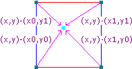
Additionally, for each of the 4 corners, the distance vector from each corner to P is calculated. These 2D vectors, illustrated below, point from each corner to P and should therefore not be normalized.
The next step is to, for each corner, calculate the dot product between the previously calculated gradient and distance vector. Congratulations, the value of this dot product is the perlin noise value of the corresponding corner. However, the goal was to calculate the perlin noise value in P instead, so you still need to do a 2D interpolation between the perlin noise values of the corners. In pseudocode:
float p00, p10, p01, p11; // the perlin noise of the
                          // 4 corners (x0,y0) (x1,y0) (x0,y1) (x1,y1)
float u = x - x0; // the x value of P within the unit square
float v = y - y0; // the y value of P within the unit square
float i0 = interpolate(p00, p10, u);
float i1 = interpolate(p01, p11, u);
float perlin_P = interpolate(i0, i1, v);
// perlin_p is the perlin noise value for P = (x,y)
For now, that's it, you have calculated the perlin noise value in point P. Sections 2.3.1 and 2.3.2 go into more detail on how functions g and interpolate are chosen. Ken Perlin also included some speed optimizations in his original publications, e.g. pre-computing a table of gradient vectors and a permutation to pick vectors out of this table at random. This is out of scope for this assignment.
3.1 Choosing g
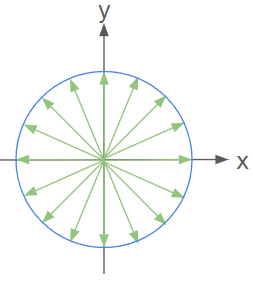
To reiterate, function g takes as input a 2D point (x,y) and should output a normalized 2D vector g(x,y) = (X,Y). The vector g(x,y) should point in a pseudo-random direction. Each direction should be equally likely. In other words, the chance of outputting any of these green vectors should be equal (of course, in our case there are infinite green arrows):
So what mathematical formula do we use for g? That is up to you to decide. Multiple solutions are viable.
One hint we will give is a function pseudo_rand that takes as input a 2D point (x,y) and outputs a pseudo-random value:
pseudo\\_rand(x,y) = fract( sin( (x, y) \cdot (12.9898, 78.233)) * 43758.5453)
Note: "pseudo-random" has a double meaning in this context:
the function does not output a perfectly random distribution, which is true for all software random number generators.
the value of
pseudo\\_rand(x',y')will not change when repeatedly called with the same(x',y').These statements should also hold for your implementation of
g.
Hopefully you will be able to make good use of pseudo_rand in g.
3.2 Choosing interpolate
You could use linear interpolation (lerp):
lerp(a, b, t) = a(1-t) + bt
but Ken Perlin wanted to create smoother, more natural looking noise. He therefore added an additional step using the smooth_step function:
smooth\\_step(t) = 3t^2 - 2t^3
To conclude, the implementation of interpolate is:
interpolate(a,b,c) = lerp(a, b, smooth\\_step(t))
By plotting lerp and smooth_step, one can get an idea of how this method can be used to smoothly interpolate the perlin noise values of the 4 corners surrounding P.
<src="docs/implementation3.png" title="" alt="implementation step 3" data-align="center">
4 Assignment
In this assignment, you will implement the generation of a 2D perlin noise texture image (resolution 512×512) on the GPU using the C++ OpenCL wrapper. The code in this repository already contains an example GPGPU program (loosely based on this tutorial) called simple_add, see GpuSimpleAdd.cpp and Addition.cl. You can run it as, for example, gpgpu.exe ..\..\src\Addition.cl. You are allowed to re-use and alter code from this example (from the .cpp , h and .cl files) to implement the generation of the perlin noise texture.
The code in GpuApplication::InitCL() begins by checking which OpenCL versions are supported by your platform. If you do not have a PC suitable for this assignment, please contact us. Then, GpuSimpleAdd::Run() calculates the element-wise sum of two vectors A and B on the GPU and writes the result to vector C.
If you have questions about the OpenCL API, for example about the keyword global, use your favorite search engine like this: “opencl khronos global” or check out the documentation of the OpenCL (C++) API and OpenCL C Specification.
In lab session 5, you will revisit perlin noise in OpenGL and use it to generate some interesting terrain.
Task 1: 2D perlin noise
You will work in two files, GpuPerlinNoise.cpp and PerlinNoise.cl, both contain additional instructions. In GpuPerlinNoise::Run(), you need to
-
Initialize the host (
vectors) and device memory (cl::Buffers) that will be necessary to store the inputs and outputs for the perlin noise algorithm. -
Launch the kernel on the device to calculate the perlin noise for 512 × 512 pixels and read the result (
output_noisefromPerlinNoise.cl) into RAM.
You may assume (i.e. hard-code) a fixed workgroup size of 16×16 threads per workgroup. From this, you can calculate the total number of workgroups. All these numbers will be important to initialize the cl::EnqueueArgs and implement perlin_noise_texture().
To calculate the gradient vectors in PerlinNoise.cl, you should implement and use the helper functions random_direction() (which corresponds to g) andpseudo_rand(), as discussed in Section 2.3.1.
Running the program, for example gpgpu.exe ..\..\src\PerlinNoise.cl will visualize the values in outputNoise as a sort of 2D terrain, see docs/perlin_terrain.gif. Use the arrow keys to rotate the scene.
Task 2: writing the perlin noise to an 8-bit image
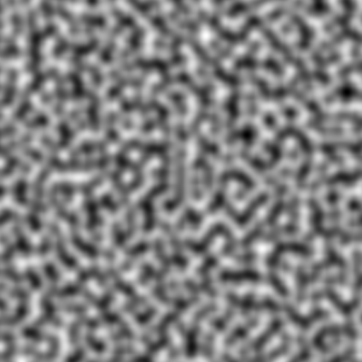
In the previous section, you will have calculated a floating-point value output_noise for each pixelId. To save the perlin noise as an 8-bit image, the values need to be converted to unsigned chars, i.e. to whole integers in [0, 255]. You could just calculate the lowest and highest value of the whole output_noise array on the CPU and then normalize all values into this range on the CPU. But this is a GPU lab, so you will try to do as much work as possible on the GPU.
Step 1: find the min and max of the output_noises within each workgroup. Remember how threads within each workgroup can share data. For each workgroup, the min and max should be written to workgroup_min[workgroupId] and workgroup_max[workgroupId] respectively.
Note: this lab is not about implementing the most efficient sorting algorithm. You are allowed to just let 1 thread per workgroup calculate the min and max of the 16×16 output_noise values of that workgroup.
Step 2: find the global min and max, i.e. over the whole image. This will not be possible on the GPU and can therefore be done on the CPU (in GpuPerlinNoise::Run()). The reason is that sharing of data across workgroups in not possible. Often, many more workgroups need to be launched than the hardware can handle at the same time, so OpenCL cannot guarantee that sharing data between workgroups will reasonably work.
Step 3: the perlin noise values, which are floating point values in [min, max], need to be scaled to fit into [0, 255] and rounded to unsigned chars. Now they are ready to be written to an 8-bit PNG texture. This whole step must be executed on the CPU in GpuPerlinNoise::Run().
Epilogue: problems with the original perlin noise implementation
So, you have implemented the original perlin noise, congratulations! Chances are that you have noticed a certain artefact. The left image below is an exaggeration of this artefact, that reveals the grid on which the perlin noise is based. This is not the only problem with the original implementation. In 2002, Ken Perlin published improved perlin noise (right image below), which makes two changes.


Improvement 1: the smooth\\_step function is swapped out with one that gives the perlin noise a continuous second derivative. This makes perlin noise more suitable for applications like bump mapping (tangents require the second derivative). Additionally, this solves the artefact discussed above.
improved\\_smooth\\_step(t) = 6t^5 - 15t^4 + 10t^3
Improvement 2: the gradient vectors being pseudo-random was not ideal. It would lead to high noise values when neighboring vectors were aligned. Instead, the gradient vectors are randomly chosen out of (1, 1, 0), (−1, 1, 0), (1,−1, 0), (−1,−1, 0), (1, 0, 1), (−1, 0, 1), (1, 0,−1), (−1, 0,−1), (0, 1, 1), (0,−1, 1), (0, 1,−1), (0,−1,−1).
Note that Ken Perlin also published simplex noise in 2001. Simplex noise is computationally more performant than perlin noise (especially for higher dimensions) and has no noticeable directional artefacts. Although being faster to compute, simplex noise is far less widespread. It is perceived to be more complex, but it is not that bad, so do not be intimidated should you ever want to use it in your own applications.
Frequently reoccuring questions/problems
-
How does OpenCL choose which device to run PerlinNoiseKernel.cl on?
Important:
main.cppcontains the following line:int idxOfPlatformAndDevice = 0;You need to set this parameter to choose which platform (that supports some version of OpenCL) you would like to use. For example, running
perlin-noise.exeshows:Found the following platforms and devices: - Platform name: NVIDIA CUDA Platform version: OpenCL 3.0 CUDA Device name: NVIDIA GeForce GTX - Platform name: Intel(R) OpenCL HD Graphics Platform version: OpenCL 2.1 Device name: Intel(R) UHD Graphics Picked combination 0, i.e. NVIDIA CUDA, OpenCL 3.0 CUDA NVIDIA GeForce GTXhere,
idxOfPlatformAndDevice = 0picked the first platform. -
The following syntax allocates an array of floats on the stack:
float A[262144];This will cause problems, since that is way too many bytes to fit on the stack. Allocate memory on the heap instead or use
std::vector. -
If your code is not working correctly and you don't know why, debug smart:
-
add print statements to main.cpp
-
try and implement parts on the CPU first and then move them to the GPU.
-
start from a simple kernel program like
simple_add()and slowly build up.
-
-
While you are implementing, feel free to add methods and play around with OpenCL. However, to hand in, make sure that the definitions of the methods are unaltered.
-
There is no "correct_results" folder, since different implementations of
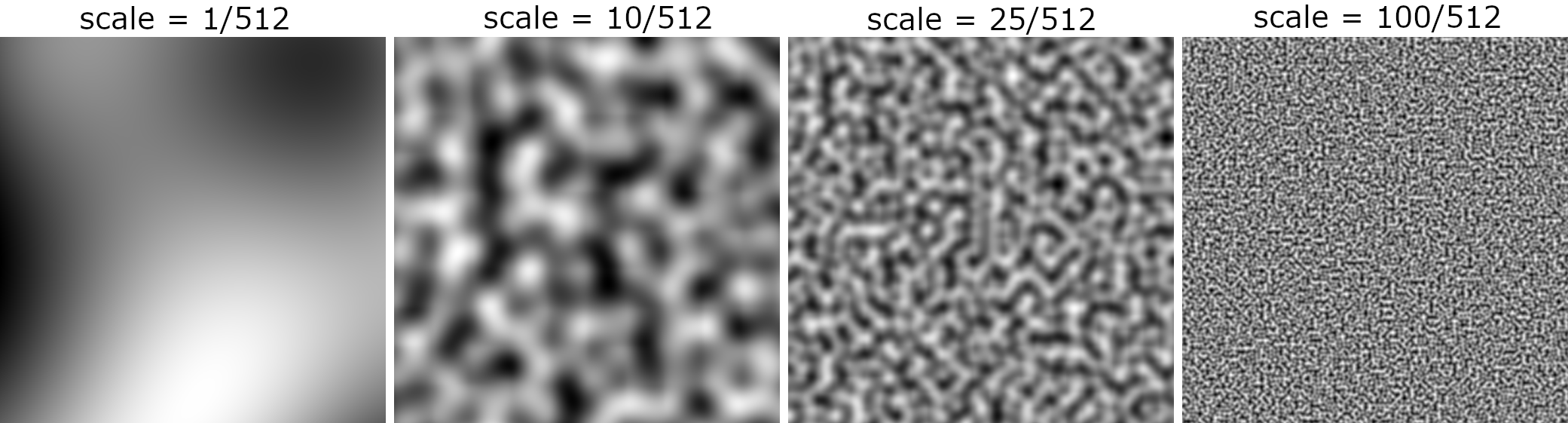
random_directionare viable but will result in different textures. Some examples are shown in the next point though. -
In
perlin_noise_texture(), the variablescaleis defined as:const float scale = 0.05f;Question: how are
(row,col)mapped to the(x,y)ofP?This determines how zoomed in your texture will be. Feel free to play with different values. Some examples:
Assignment 2: Particle system for a simplified fluid

Particle simulation is a good example of something that is best implemented using GPGPU. In GpuParticleSystem.cpp and ParticleSystem.cl, you will implement the simplified, two-dimensional liquid simulation shown above using particles. You will use OpenCL to update the position (and velocity) of each particle, for every frame. Afterwards, these positions (and velocities) are passed to OpenGL, which draws each particle as a point on screen. The color of each particle changes with its speed.
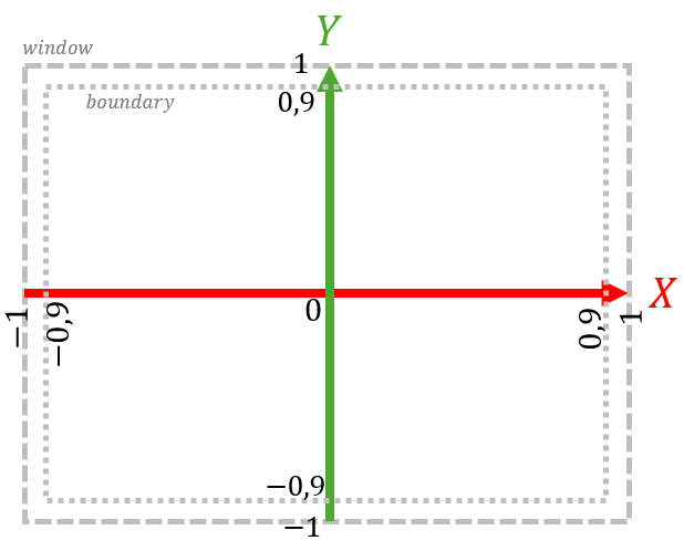
Take a look at the vectors positions and velocities in GpuParticleSystem.cpp. They each contain 2*nrParticles floats, since we are working in 2D. For example, if nrParticles == 2, then positions = {x0, y0, x1, y1}. This begs the question: where are the X and Y axes, and where lie the boundaries of the container to which the liquid is confined? We will use OpenGL's "Normalized device coordinate" (NDC) axial system: (x,y)∈ [-1, 1]², with the X-axis pointing to the right, and the Y-axis pointing upwards. The boundaries of the liquid should be [-0.9, 0.9]². So, regardless of the resolution or aspect ratio of the window, the NDC space will look like this:
Whenever you come across // your code here in GpuParticleSystem.cpp and ParticleSystem.cl, you will have to implement something. More specifically, in GpuParticleSystem.cpp, the following features are expected:
-
GpuParticleSystem::InitPosVel(): initialize the positions and velocities of each particle. Run for examplegpgpu.exe ..\..\src\ParticleSystem.clto visualize. -
GpuParticleSystem::Run(): setup the OpenCL kernel fromParticleSystem.cl, so thatupdateParticles()can be called. Use 1 thread per particle. You can useGpuSimpleAdd.cppas inspiration. In thewhile-loop, call the kernel to update the particles and download the results back to the CPU, intopositionsandvelocities. Use OpenGL'sglBindBuffer()andglBufferSubData()to overwrite OpenGL's VBOs with the newpositionsandvelocities(OpenGL is quite well documented). -
When running
gpgpu.exe, and pressingron your keyboard,HandleUserInput()will setreset = true, which will callInitPosVel()to reset the simulation. Make sure that the OpenCLcl::Buffers are updated accordingly.
Simultaneously, ParticleSystem.cl should have the following features:
-
Get the index of the current thread, and thus the indices of the current particle in the
positionsandvelocitiesarrays. UseAddition.clas inspiration. You will only need to update the 2D position and velocity of this 1 particle. -
At the end of
updateParticles(), thepositionof the particle should be updated using itsvelocityanddt(= the duration of 1 frame, in seconds). Hopefully you still remember how to update a position based on the velocity, and the velocity based on the acceleration, and a small timestep (dt). -
Just before this, the velocity should be dampened as follows:
velocity *= damping, to prevent particles from moving forever. This is a simplified way of implementing friction forces. -
The particle should be affected by gravity. Use
g = 9.8 m/s²(assuming that the NDC is defined in meters). -
Several repulsion forces should work on the particle. Note however, that
force = mass * acceleration, but we neglect mass here, so instead of appling N "forces" on the particle, we will apply N acceleration vectors, which, when all summed up, will change thevelocities(usingdt).-
The particle should stay within the boundary box
[-0.9, 0.9]². To implement this, first, when a particle crosses a boundary, it should be teleported back to the correct side of the boundary, and the velocity along this axis should be reset to 0. Secondly, if a particle is withinboundaryRepulsionRadiusof a boundary, a repulsion force should be added, pointed away from the boundary. The acceleration should increase according to a parabole (f(x) = x²):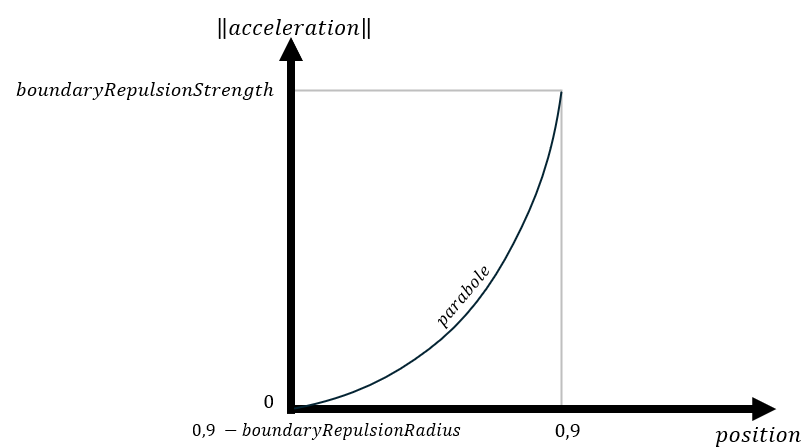
-
The particle should be repelled from other particles within
repulsionRadius. Similarly to the previous point, you can userepulsionRadiusandrepulsionStrength. Instead of a parabole, you can simply make the norm of the acceleration vector increase linearly with the closeness to the other particle. -
The particle should be repelled from the cursor. You can reuse
boundaryRepulsionRadiusandboundaryRepulsionStrength.
-
Some remarks:
- It can be helpful to disable certain features of
updateParticles()while implementing others. For example, disable the gravity. - You don't need to worry about memory barriers in
updateParticles(). - At the beginning of the simulation, the particles rapidly get pushed away from eachother. This is just a simplified fluid simulation, improving the realism here is out-of-scope for this assignment.
- Right now, in every thread, you are looping over every particle and calculate distances. Optimizations exist, but they are out-of-scope.
- Right now, for every frame, you download
positionsandvelocitiesfrom GPU->CPU and then upload it again CPU->GPU. It is definitely possible (and recommended) to skip this step, and simply use a buffer located on the GPU that can be accessed by both the OpenCL and OpenGL context. This is often denoted as an "interop" between OpenCL and OpenGL. However, this is no OpenGL lab, so this is out-of-scope.