[](https://classroom.github.com/a/Po9MPlbW)
# Computer Graphics Lab3 – Meshes
**Deadline: Nov. 15 2024, 22:00**
## Building using CMake
### Windows
If your CMake version < 3.16.0, you might see an error pop up while using CMake, saying that Libigl requires a version >= 3.16.0. If you don't want to update your CMake, simply go to the line throwing that error and change the version:
```
# on my machine the error is thrown in
# "out/build/x64-Debug/_deps/libigl-src/CMakeLists.txt" on line 12:
set(REQUIRED_CMAKE_VERSION "3.16.0")
# change this to a version <= your version, for example:
set(REQUIRED_CMAKE_VERSION "3.0.0")
```
### Linux
If CMake succeeds without errors, great. However, if not, then you will have to resolve the thrown exceptions. We follow [libigl's example project](https://github.com/libigl/libigl-example-project) in this assignment, which they claim should work on Ubuntu out of the box. It can be however that CMake throws exceptions that look like:
1. `"Could not find X11 (missing: X11_X11_LIB ...)"`
2. `"... headers not found; ... install ... development package"`
3. `"Could NOT find OpenGL (missing: OPENGL_opengl_LIBRARY ...)"`
To solve errors like this, install the missing packages (you might need to search around on the web if the following command does not suffice):
```
sudo apt install libx11-dev libxrandr-dev libxinerama-dev libxcursor-dev libxi-dev libgl1-mesa-dev
```
### WSL (Windows)
Follow the Linux instructions above. Warning: the assignment uses OpenGL and GLFW to create a window, which might not work with WSL. We will not be able to help you here.
### MacOS
We follow [libigl's example project](https://github.com/libigl/libigl-example-project) in this assignment, which they claim should work on MacOS out of the box. If you experience CMake errors that you cannot solve with some help online, please contact us.
## Background
### Read Section 12.1 of _Fundamentals of Computer Graphics (4th Edition)_.
### Skim read Chapter 11 of _Fundamentals of Computer Graphics (4th Edition)_.
There are many ways to store a triangle (or polygonal) mesh on the computer. The
data-structures have very different complexities in terms of code, memory, and
access performance. At the heart of these structures, is the problem of storing
the two types of information defining a mesh: the _geometry_ (where are points
on the surface located in space) and the _connectivity_ (which points are
connected to each other). The connectivity is also sometimes referred to as the
[topology](https://en.wikipedia.org/wiki/Topology) of the mesh.
The [graphics pipeline](https://en.wikipedia.org/wiki/Graphics_pipeline) works
on a per-triangle and per-vertex basis. So the simplest way to store geometry is
a 3D position  for each
  -th vertex of the mesh. And to store
triangle connectivity as an ordered triplet of indices referencing vertices:
-th vertex of the mesh. And to store
triangle connectivity as an ordered triplet of indices referencing vertices:
 defines a triangle with corners at vertices
  ,
,  and
and  .
Thus, the geometry is stored as a list of
.
Thus, the geometry is stored as a list of  3D vectors: efficiently, we can
put these vectors in the rows of a real-valued matrix
3D vectors: efficiently, we can
put these vectors in the rows of a real-valued matrix  . Likewise,
the connectivity is stored as a list of
. Likewise,
the connectivity is stored as a list of  triplets: efficiently, we can put
these triplets in the rows of an integer-valued matrix
triplets: efficiently, we can put
these triplets in the rows of an integer-valued matrix  .
> **Question:** What if we want to store a (pure-)quad mesh?
### Texture Mapping
[Texture mapping](https://en.wikipedia.org/wiki/Texture_mapping) is a process
for mapping image information (e.g., colors) onto a surface (e.g., triangle
mesh). The standard way to define a texture mapping is to augment the 3D
geometric information of a mesh with additional 2D _parametrization_
information: where do we find each point on the texture image plane? Typically,
parameterization coordinates are bound to the unit square.
Mapping a 3D flat polygon to 2D is rather straightforward. The problem of
finding a good mapping from a 3D surface to 2D becomes much harder if our
surface is not flat (e.g., like a
[hemisphere](https://en.wikipedia.org/wiki/Hemisphere)), if the surface does not
have exact one boundary (e.g., like a sphere) or if the surface has "holes"
(e.g., like a [torus/doughnut](https://en.wikipedia.org/wiki/Torus)).
Curved surfaces must get _distorted_ when flattened onto the plane. This is why
[Greenland looks bigger than
Africa](https://www.youtube.com/watch?v=vVX-PrBRtTY) on a common map of the
Earth.
The lack or presence of too many boundaries or the presence of "doughnut holes"
in surfaces implies that we need to "cut" the surface to lay out it on the
plane so all parts of the surface are "face up". _Think about trying to flatten
a deflated basketball on the ground._
### Normals
For a smooth surface, knowing the surface geometry (i.e., position in space)
near a point fully determines the [normal
vector](https://en.wikipedia.org/wiki/Normal_(geometry)) at that point.
For a discrete mesh, the normal is only well-defined in the middle of planar
faces (e.g., inside the triangles of a triangle mesh, but not along the edges or
at vertices). Furthermore, if we use these normals for rendering, the surface
will have a faceted appearance. This appearance is mathematically correct, but
not necessarily desired if we wish to display a smooth looking surface.
[Phong](https://en.wikipedia.org/wiki/Bui_Tuong_Phong) realized that [linearly
interpolating](https://en.wikipedia.org/wiki/Linear_interpolation) normals
stored at the corners of each triangle leads to a [smooth
appearance](https://en.wikipedia.org/wiki/Phong_shading#Phong_interpolation).
This raises the question: what normals should we put at vertices or corners of
our mesh?
For a faceted surface (e.g., a cube), all corners of a planar face
.
> **Question:** What if we want to store a (pure-)quad mesh?
### Texture Mapping
[Texture mapping](https://en.wikipedia.org/wiki/Texture_mapping) is a process
for mapping image information (e.g., colors) onto a surface (e.g., triangle
mesh). The standard way to define a texture mapping is to augment the 3D
geometric information of a mesh with additional 2D _parametrization_
information: where do we find each point on the texture image plane? Typically,
parameterization coordinates are bound to the unit square.
Mapping a 3D flat polygon to 2D is rather straightforward. The problem of
finding a good mapping from a 3D surface to 2D becomes much harder if our
surface is not flat (e.g., like a
[hemisphere](https://en.wikipedia.org/wiki/Hemisphere)), if the surface does not
have exact one boundary (e.g., like a sphere) or if the surface has "holes"
(e.g., like a [torus/doughnut](https://en.wikipedia.org/wiki/Torus)).
Curved surfaces must get _distorted_ when flattened onto the plane. This is why
[Greenland looks bigger than
Africa](https://www.youtube.com/watch?v=vVX-PrBRtTY) on a common map of the
Earth.
The lack or presence of too many boundaries or the presence of "doughnut holes"
in surfaces implies that we need to "cut" the surface to lay out it on the
plane so all parts of the surface are "face up". _Think about trying to flatten
a deflated basketball on the ground._
### Normals
For a smooth surface, knowing the surface geometry (i.e., position in space)
near a point fully determines the [normal
vector](https://en.wikipedia.org/wiki/Normal_(geometry)) at that point.
For a discrete mesh, the normal is only well-defined in the middle of planar
faces (e.g., inside the triangles of a triangle mesh, but not along the edges or
at vertices). Furthermore, if we use these normals for rendering, the surface
will have a faceted appearance. This appearance is mathematically correct, but
not necessarily desired if we wish to display a smooth looking surface.
[Phong](https://en.wikipedia.org/wiki/Bui_Tuong_Phong) realized that [linearly
interpolating](https://en.wikipedia.org/wiki/Linear_interpolation) normals
stored at the corners of each triangle leads to a [smooth
appearance](https://en.wikipedia.org/wiki/Phong_shading#Phong_interpolation).
This raises the question: what normals should we put at vertices or corners of
our mesh?
For a faceted surface (e.g., a cube), all corners of a planar face  should
share the face's normal
should
share the face's normal  .
For a smooth surface (e.g., a sphere), corners of triangles located at the same
vertex should share the same normal vector. This way the rendering is continuous
across the vertex. A common way to define per-vertex normals is to take a
weighted average of normals from incident faces. Different weighting schemes are
possible: uniform average (easy, but sensitive to irregular triangulations),
angle-weighted (geometrically well motivated, but not robust near zero-area
triangles), area-weighted (geometrically reasonable, well behaved). In this
assignment, we'll compute area-weighted per-vertex normals:
.
For a smooth surface (e.g., a sphere), corners of triangles located at the same
vertex should share the same normal vector. This way the rendering is continuous
across the vertex. A common way to define per-vertex normals is to take a
weighted average of normals from incident faces. Different weighting schemes are
possible: uniform average (easy, but sensitive to irregular triangulations),
angle-weighted (geometrically well motivated, but not robust near zero-area
triangles), area-weighted (geometrically reasonable, well behaved). In this
assignment, we'll compute area-weighted per-vertex normals:

where  is the set of faces neighboring the
  -th vertex.
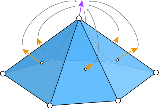
For surfaces with a mixture of smooth-looking parts and creases, it is useful to
define normals independently for each triangle corner (as opposed to each mesh
vertex). For each corner, we'll again compute an area-weighted average of normals
triangles incident on the shared vertex at this corner, but we'll ignore
triangle's whose normal is too different from the corner's face's normal:
-th vertex.

For surfaces with a mixture of smooth-looking parts and creases, it is useful to
define normals independently for each triangle corner (as opposed to each mesh
vertex). For each corner, we'll again compute an area-weighted average of normals
triangles incident on the shared vertex at this corner, but we'll ignore
triangle's whose normal is too different from the corner's face's normal:

where  is the minimum dot product between two face normals before we declare
there is a crease between them.

### .obj File Format
A common file format to save meshes is the [.obj file format](https://en.wikipedia.org/wiki/Wavefront_.obj_file), which contains a _face_-based representation. The connectivity/topological data is stored implicitly by a list of faces made out of vertices. Per vertex, three main types of geometric information can be stored:
- 3D position information of a vertex (denoted as `v` in the file, and `V` in the src code)
- 3D normal vector information of a vertex (`vn`, or `NV` in src code)
- 2D parameterization information (e.g. texture coordinate) of a vertex (`vt`, or `UV` in the src code)
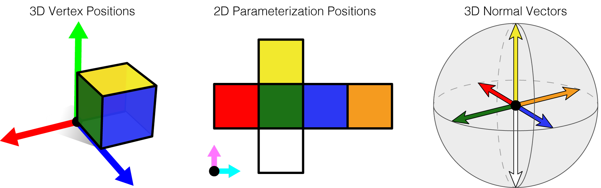
Take a cube for example. You could construct a mesh with 6 faces, each having 1 normal vector, and 4 vertices per face. You could make it so that each vertex has a 2D texture coordinate.
In an .obj file, a face is defined as a list of indices pointing towards certain lines of `v`, `vt` and/or `vn`. For example :
```
v 0.0 0.0 0.0 # 3D position 1
v 2.0 0.0 0.0 # 2
v 1.0 2.0 0.0 # 3
vt 0.0 0.0 # 2D texture coordinate 1
vt 1.0 0.0 # 2
vt 0.5 1.0 # 3
vn 0.0 0.0 1.0 # 3D normal vector 1
# some examples faces that can be made:
f 1 2 3 # face 1: a face made of 3 vertices, with 3D positions 1,2,3
f 1/1 2/2 3/3 # face 2: same as face 1, but with 2D texture coordinates 1,2,3 respectively
f 1//1 2//1 3//1 # face 3: same as face 1, but with normal vector 1 for each vertex
f 1/1/1 2/2/1 3/3/1 # face 4: each vertex has a position, texture coordinate and normal vector
```
> **Warning:** In an .obj file, indexing always starts at `1`, not `0`!
This is just an example of course. Faces can have more than 3 vertices, can have vertices with different normal vectors, and the order of faces does not matter.
### Subdivision Surfaces
A [subdivision surface](https://en.wikipedia.org/wiki/Subdivision_surface) is a
natural generalization of a [spline
curve](https://en.wikipedia.org/wiki/Spline_(mathematics)). A smooth spline can
be defined as the [limit](https://en.wikipedia.org/wiki/Limit_(mathematics)) of
a [recursive
process](https://en.wikipedia.org/wiki/Recursion_(computer_science)) applied to
a polygon: each edge of the polygon is split with a new vertex and the vertices
are smoothed toward eachother. If you've drawn smooth curves using Adobe
Illustrator, PowerPoint or Inkscape, then you've used splines.
At a high-level, subdivision surfaces work the same way. We start with a
polyhedral mesh and subdivide each face. This adds new vertices on the faces
and/or edges of the mesh. Then we smooth vertices toward each other.
The first and still (most) popular subdivision scheme was invented by
[Catmull](https://en.wikipedia.org/wiki/Edwin_Catmull) (who went on to co-found
[Pixar](https://en.wikipedia.org/wiki/Pixar)) and
[Clark](https://en.wikipedia.org/wiki/James_H._Clark) (founder of
[Silicon Graphics](https://en.wikipedia.org/wiki/Silicon_Graphics) and
[Netscape](https://en.wikipedia.org/wiki/Netscape)). [Catmull-Clark
subdivision](https://en.wikipedia.org/wiki/Catmull–Clark_subdivision_surface) is
defined for inputs meshes with arbitrary polygonal faces (triangles, quads,
pentagons, etc.) but always produces a pure-quad mesh as output (i.e., all faces
have 4 sides).
To keep things simple, in this assignment we'll assume the input is also a
pure-quad mesh.
 converging
toward a smooth surface.](markdown/bob-subdivision.gif)
## Mesh Viewers
(Optional) In this assignment, you will create meshes that you can save to an .obj file thanks to `write_obj.cpp`. If you would like to view these meshes in something other than the `libigl` viewer we provide, you can open the .obj files in:
1. [Mesh Lab](http://www.meshlab.net) free, open-source. **_Warning_:** Mesh Lab does not appear
to respect user-provided normals in .obj files.
2. [Blender](https://www.blender.org/download/): free, open-source. If you want to see the texture, you will have to make a shader with an image texture.
3. [Autodesk Maya](https://en.wikipedia.org/wiki/Autodesk_Maya) is a commericial 3D
modeling and animation software. They often have [free student versions](https://www.autodesk.com/education/free-software/maya).
## Almost ready to start implementing
### Eigen Matrices
This assignment use the Eigen library. This section contains some useful syntax:
```
Eigen::MatrixXi A; // creates a 0x0 matrix of integers
A.resize(10, 3); // resizes the matrix to 10x3 (meaning 10 rows, 3 columns)
Eigen::MatrixXd B; // creates a 0x0 matrix of doubles
B.resize(10, 3); // important, always use resize() !
Eigen::MatrixXd C = Eigen::MatrixXd::Zero(10, 3); // here C.resize() is not necessary
C.row(0) = Eigen::RowVector3d(0, 0, 1); // overwrite the first row of C
C.row(5); // gives the 5th row of C, as an Eigen::RowVectorXd
C(5,0); // gives the element on row=5 and column=0 of C
```
### White list
You're encouraged to use `#include ` to compute the [cross
product](https://en.wikipedia.org/wiki/Cross_product) of two 3D vectors
`.cross`.
### Black list
This assignment uses [libigl](http://libigl.github.io) for mesh viewing. libigl
has many mesh processing functions implemented in C++, including some of the
functions assigned here. Do not copy or look at the following implementations:
`igl::per_vertex_normals`
`igl::per_face_normals`
`igl::per_corner_normals`
`igl::double_area`
`igl::vertex_triangle_adjacency`
`igl::writeOBJ`
# Tasks
## Part 1: Understanding the .OBJ File Format
Once you have implemented the files below, run
```
Linux: ./obj ../data/rubiks-cube.png ../data/earth-square.png
Windows: obj.exe ../../../data/rubiks-cube.png ../../../data/earth-square.png
```
to open a window showing your cube being rendered. If you press 'Escape', it will close and the second window displaying your sphere will pop up. They should look like this:
](markdown/rubiks-cube.gif)
> Tip: look at the **header file** of each function to implement.
### `src/write_obj.cpp`
The input is a mesh with
1. 3D vertex positions (`V`)
2. 2D parametrization positions (`UV`)
3. 3D normal vectors (`NV`)
4. the vertices making up the faces (`F`), denoted as indices of `V`
5. the uvs of the faces (`UF`), denoted as indices of `UV`
5. the normal vectors of the faces (`UF`), denoted as indices of `NV`
The goal is to write the mesh to an `.obj` file.
> **Note:** This assignment covers only a small subset of meshes and mesh-data that the `.obj` file format supports.
### `src/cube.cpp`
Construct the **quad** mesh of a cube including parameterization and per-face
normals.
> **Hint:** Draw out on paper and _label_ with indices the 3D cube, the 2D
> parameterized cube, and the normals.
### `src/sphere.cpp` (optional, not included in rating)
Construct a **quad** mesh of a sphere with `num_faces_u` × `num_faces_v` faces. Take a look at UV spheres or [equirectangular projection/mapping](https://www.youtube.com/watch?v=15dVTZg0rhE).
The equirectangular projection basically defines how a 3D vertex `(x,y,z)` on the sphere is mapped to a 2D texture coordinate `(u,v)`, and vice versa. To go from `(u,v)` to `(x,y,z)` (although some flipping of axes might be necessary):
```
φ = 2π - 2πu # φ is horizontal and should go from 2π to 0 as u goes from 0 to 1
θ = π - πv # θ is vertical and should go from π to 0 as v goes from 0 to 1
x = sin(θ)cos(φ)
y = cos(θ)
z = sin(θ)sin(φ)
```
> **Note**: The `v` axis of the texture coordinate is always upwards
## Part 2: Calculating normal vectors
You may assume that the input .obj files will all contain faces with 3 vertices (triangles), like `fandisk.obj`. Once you have implemented the functions below, run
```
Linux: ./normals ../data/fandisk.obj
Windows: normals.exe ../../../data/fandisk.obj
```
to open a window showing the fandisk being rendered using the normals calculated by you. Type '1', '2' or '3' (above qwerty/azerty on the keyboard) to switch between per-face, per-vertex and per-corner normals. The difference between per-face and per-corner is only visible when zoomed in.
> Tip: look at the **header file** of each function to implement.
### `src/triangle_area_normal.cpp`
Compute the normal vector of a 3D triangle given its corner locations. The
output vector should have length equal to the area of the triangle.
**Important**: this the only time where you are allowed to return normal vectors that do not have unit length (i.e. that have not been normalized).
### `src/per_face_normals.cpp`
Compute per-face normals for a triangle mesh. In other words: for each face, compute the normal vector **of unit length**.
### `src/per_vertex_normals.cpp`
Compute per-vertex normals for a triangle mesh. In other words: for each vertex, compute the normal vector **of unit length**, by taking a area-weighted average over the normals of all the faces with that vertex as a corner.
### `src/vertex_triangle_adjacency.cpp`
Compute a vertex-triangle adjacency list. For each vertex store a list of all incident faces. Tip: `emplace_back()`.
### `src/per_corner_normals.cpp`
Compute per-corner normals for a triangle mesh. The goal is to compute a **unit** normal vector for each corner C of each face F. This is done by taking the area-weighted average of normals of faces connected to C. However, an incident face's normals is only included in the area-weighted average if the angle between that face normal and that of F is smaller than a threshold (`corner_threshold` (= 20 degrees)).
## Part 3: Implementing a mesh subdivision method
### `src/catmull_clark.cpp`
Conduct `num_iters` iterations of [Catmull-Clark
subdivision](https://en.wikipedia.org/wiki/Catmull–Clark_subdivision_surface) on
a **pure quad** mesh (`V`,`F`).
Once this is implemented, run `./quad_subdivision` (or `quad_subdivision.exe`) on your `cube.obj` or `bob.obj` (shown earlier). Press 'spacebar' to subdivide once. It should look nicely smooth and uniform from all sides:

> Tip: First get cube.obj working before moving onto bob.obj.
> Tip: I think the step-by-step explanation on [Wikipedia (under "Recursive evaluation")](https://en.wikipedia.org/wiki/Catmull%E2%80%93Clark_subdivision_surface) is quite clear.
> Tip: **perform the Catmull-Clark algorithm on paper first**, i.e. draw the cube from cube.obj on a piece of paper and manually calculate each `face point`, `edge point` and `new vertex point`. Check if these values are the same as your implementation.
is the minimum dot product between two face normals before we declare
there is a crease between them.

### .obj File Format
A common file format to save meshes is the [.obj file format](https://en.wikipedia.org/wiki/Wavefront_.obj_file), which contains a _face_-based representation. The connectivity/topological data is stored implicitly by a list of faces made out of vertices. Per vertex, three main types of geometric information can be stored:
- 3D position information of a vertex (denoted as `v` in the file, and `V` in the src code)
- 3D normal vector information of a vertex (`vn`, or `NV` in src code)
- 2D parameterization information (e.g. texture coordinate) of a vertex (`vt`, or `UV` in the src code)
Take a cube for example. You could construct a mesh with 6 faces, each having 1 normal vector, and 4 vertices per face. You could make it so that each vertex has a 2D texture coordinate.

In an .obj file, a face is defined as a list of indices pointing towards certain lines of `v`, `vt` and/or `vn`. For example :
```
v 0.0 0.0 0.0 # 3D position 1
v 2.0 0.0 0.0 # 2
v 1.0 2.0 0.0 # 3
vt 0.0 0.0 # 2D texture coordinate 1
vt 1.0 0.0 # 2
vt 0.5 1.0 # 3
vn 0.0 0.0 1.0 # 3D normal vector 1
# some examples faces that can be made:
f 1 2 3 # face 1: a face made of 3 vertices, with 3D positions 1,2,3
f 1/1 2/2 3/3 # face 2: same as face 1, but with 2D texture coordinates 1,2,3 respectively
f 1//1 2//1 3//1 # face 3: same as face 1, but with normal vector 1 for each vertex
f 1/1/1 2/2/1 3/3/1 # face 4: each vertex has a position, texture coordinate and normal vector
```
> **Warning:** In an .obj file, indexing always starts at `1`, not `0`!
This is just an example of course. Faces can have more than 3 vertices, can have vertices with different normal vectors, and the order of faces does not matter.
### Subdivision Surfaces
A [subdivision surface](https://en.wikipedia.org/wiki/Subdivision_surface) is a
natural generalization of a [spline
curve](https://en.wikipedia.org/wiki/Spline_(mathematics)). A smooth spline can
be defined as the [limit](https://en.wikipedia.org/wiki/Limit_(mathematics)) of
a [recursive
process](https://en.wikipedia.org/wiki/Recursion_(computer_science)) applied to
a polygon: each edge of the polygon is split with a new vertex and the vertices
are smoothed toward eachother. If you've drawn smooth curves using Adobe
Illustrator, PowerPoint or Inkscape, then you've used splines.
At a high-level, subdivision surfaces work the same way. We start with a
polyhedral mesh and subdivide each face. This adds new vertices on the faces
and/or edges of the mesh. Then we smooth vertices toward each other.
The first and still (most) popular subdivision scheme was invented by
[Catmull](https://en.wikipedia.org/wiki/Edwin_Catmull) (who went on to co-found
[Pixar](https://en.wikipedia.org/wiki/Pixar)) and
[Clark](https://en.wikipedia.org/wiki/James_H._Clark) (founder of
[Silicon Graphics](https://en.wikipedia.org/wiki/Silicon_Graphics) and
[Netscape](https://en.wikipedia.org/wiki/Netscape)). [Catmull-Clark
subdivision](https://en.wikipedia.org/wiki/Catmull–Clark_subdivision_surface) is
defined for inputs meshes with arbitrary polygonal faces (triangles, quads,
pentagons, etc.) but always produces a pure-quad mesh as output (i.e., all faces
have 4 sides).
To keep things simple, in this assignment we'll assume the input is also a
pure-quad mesh.
 converging
toward a smooth surface.](markdown/bob-subdivision.gif)
## Mesh Viewers
(Optional) In this assignment, you will create meshes that you can save to an .obj file thanks to `write_obj.cpp`. If you would like to view these meshes in something other than the `libigl` viewer we provide, you can open the .obj files in:
1. [Mesh Lab](http://www.meshlab.net) free, open-source. **_Warning_:** Mesh Lab does not appear
to respect user-provided normals in .obj files.
2. [Blender](https://www.blender.org/download/): free, open-source. If you want to see the texture, you will have to make a shader with an image texture.
3. [Autodesk Maya](https://en.wikipedia.org/wiki/Autodesk_Maya) is a commericial 3D
modeling and animation software. They often have [free student versions](https://www.autodesk.com/education/free-software/maya).
## Almost ready to start implementing
### Eigen Matrices
This assignment use the Eigen library. This section contains some useful syntax:
```
Eigen::MatrixXi A; // creates a 0x0 matrix of integers
A.resize(10, 3); // resizes the matrix to 10x3 (meaning 10 rows, 3 columns)
Eigen::MatrixXd B; // creates a 0x0 matrix of doubles
B.resize(10, 3); // important, always use resize() !
Eigen::MatrixXd C = Eigen::MatrixXd::Zero(10, 3); // here C.resize() is not necessary
C.row(0) = Eigen::RowVector3d(0, 0, 1); // overwrite the first row of C
C.row(5); // gives the 5th row of C, as an Eigen::RowVectorXd
C(5,0); // gives the element on row=5 and column=0 of C
```
### White list
You're encouraged to use `#include ` to compute the [cross
product](https://en.wikipedia.org/wiki/Cross_product) of two 3D vectors
`.cross`.
### Black list
This assignment uses [libigl](http://libigl.github.io) for mesh viewing. libigl
has many mesh processing functions implemented in C++, including some of the
functions assigned here. Do not copy or look at the following implementations:
`igl::per_vertex_normals`
`igl::per_face_normals`
`igl::per_corner_normals`
`igl::double_area`
`igl::vertex_triangle_adjacency`
`igl::writeOBJ`
# Tasks
## Part 1: Understanding the .OBJ File Format
Once you have implemented the files below, run
```
Linux: ./obj ../data/rubiks-cube.png ../data/earth-square.png
Windows: obj.exe ../../../data/rubiks-cube.png ../../../data/earth-square.png
```
to open a window showing your cube being rendered. If you press 'Escape', it will close and the second window displaying your sphere will pop up. They should look like this:
](markdown/rubiks-cube.gif)

> Tip: look at the **header file** of each function to implement.
### `src/write_obj.cpp`
The input is a mesh with
1. 3D vertex positions (`V`)
2. 2D parametrization positions (`UV`)
3. 3D normal vectors (`NV`)
4. the vertices making up the faces (`F`), denoted as indices of `V`
5. the uvs of the faces (`UF`), denoted as indices of `UV`
5. the normal vectors of the faces (`UF`), denoted as indices of `NV`
The goal is to write the mesh to an `.obj` file.
> **Note:** This assignment covers only a small subset of meshes and mesh-data that the `.obj` file format supports.
### `src/cube.cpp`
Construct the **quad** mesh of a cube including parameterization and per-face
normals.
> **Hint:** Draw out on paper and _label_ with indices the 3D cube, the 2D
> parameterized cube, and the normals.
### `src/sphere.cpp` (optional, not included in rating)
Construct a **quad** mesh of a sphere with `num_faces_u` × `num_faces_v` faces. Take a look at UV spheres or [equirectangular projection/mapping](https://www.youtube.com/watch?v=15dVTZg0rhE).
The equirectangular projection basically defines how a 3D vertex `(x,y,z)` on the sphere is mapped to a 2D texture coordinate `(u,v)`, and vice versa. To go from `(u,v)` to `(x,y,z)` (although some flipping of axes might be necessary):
```
φ = 2π - 2πu # φ is horizontal and should go from 2π to 0 as u goes from 0 to 1
θ = π - πv # θ is vertical and should go from π to 0 as v goes from 0 to 1
x = sin(θ)cos(φ)
y = cos(θ)
z = sin(θ)sin(φ)
```
> **Note**: The `v` axis of the texture coordinate is always upwards
## Part 2: Calculating normal vectors
You may assume that the input .obj files will all contain faces with 3 vertices (triangles), like `fandisk.obj`. Once you have implemented the functions below, run
```
Linux: ./normals ../data/fandisk.obj
Windows: normals.exe ../../../data/fandisk.obj
```
to open a window showing the fandisk being rendered using the normals calculated by you. Type '1', '2' or '3' (above qwerty/azerty on the keyboard) to switch between per-face, per-vertex and per-corner normals. The difference between per-face and per-corner is only visible when zoomed in.

> Tip: look at the **header file** of each function to implement.
### `src/triangle_area_normal.cpp`
Compute the normal vector of a 3D triangle given its corner locations. The
output vector should have length equal to the area of the triangle.
**Important**: this the only time where you are allowed to return normal vectors that do not have unit length (i.e. that have not been normalized).
### `src/per_face_normals.cpp`
Compute per-face normals for a triangle mesh. In other words: for each face, compute the normal vector **of unit length**.
### `src/per_vertex_normals.cpp`
Compute per-vertex normals for a triangle mesh. In other words: for each vertex, compute the normal vector **of unit length**, by taking a area-weighted average over the normals of all the faces with that vertex as a corner.
### `src/vertex_triangle_adjacency.cpp`
Compute a vertex-triangle adjacency list. For each vertex store a list of all incident faces. Tip: `emplace_back()`.
### `src/per_corner_normals.cpp`
Compute per-corner normals for a triangle mesh. The goal is to compute a **unit** normal vector for each corner C of each face F. This is done by taking the area-weighted average of normals of faces connected to C. However, an incident face's normals is only included in the area-weighted average if the angle between that face normal and that of F is smaller than a threshold (`corner_threshold` (= 20 degrees)).
## Part 3: Implementing a mesh subdivision method
### `src/catmull_clark.cpp`
Conduct `num_iters` iterations of [Catmull-Clark
subdivision](https://en.wikipedia.org/wiki/Catmull–Clark_subdivision_surface) on
a **pure quad** mesh (`V`,`F`).
Once this is implemented, run `./quad_subdivision` (or `quad_subdivision.exe`) on your `cube.obj` or `bob.obj` (shown earlier). Press 'spacebar' to subdivide once. It should look nicely smooth and uniform from all sides:

> Tip: First get cube.obj working before moving onto bob.obj.
> Tip: I think the step-by-step explanation on [Wikipedia (under "Recursive evaluation")](https://en.wikipedia.org/wiki/Catmull%E2%80%93Clark_subdivision_surface) is quite clear.
> Tip: **perform the Catmull-Clark algorithm on paper first**, i.e. draw the cube from cube.obj on a piece of paper and manually calculate each `face point`, `edge point` and `new vertex point`. Check if these values are the same as your implementation.